Developer Tenets
Open data projects like Overture are built across time. Contributors come and go, member companies rotate people in and out, and the builders of today are extending the work of those who came before them. Part of the work of Overture is documenting how we work, to help new contributors quickly get up to speed and to capture the immense technical and organizational knowledge built up over the past few years.
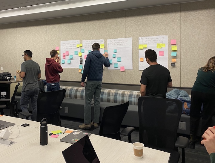 OG Overture developers from multiple organizations taking a break from coding for some analog collaboration and documentation, February 2024.
Our contributor base itself is wide. People bring code, documentation, data analysis, quality checks, and more to the project, and they come from an incredibly diverse range of organizations: big tech, scrappy startups, nonprofits, government agencies, and open data communities. This diversity is a strength, giving us a wide range of perspectives and skills. It can also create friction, since these organizations bring different goals, tools, constraints, development velocities, and cultures.
Rather than subjecting our contributors to a strict set of engineering guidelines, we want to communicate a set of higher-level values. These values should be reflected throughout the development cycle, in the documentation we write and the pull requests we post. Beyond giving developers flexibility, this approach is AI-friendly: skills and agents can use this document as broad context for testing intent.
The "Developer Tenets" below are adapted from our internal Overture operations guide. We're publishing them because they're the kind of thing that benefits from being out in the open, where contributors and downstream users can see how we think about building Overture, at least from the engineering side. The tenets were defined by the developers, and Claude helped expand them with examples and code review guidance, i.e. "what to check." That pattern (humans setting direction, AI in a supporting role) is central to how we operate.