GERS Tutorial

Why associate your data with GERS identifiers?

Overture Data isn’t just a base layer for building your own map, it’s a shared reference layer for exchanging and enriching geospatial data. The Global Entity Reference System (GERS) is the framework that enables this exchange. Every datapoint in Overture data releases has a GERS identifier, a persistent value referencing itself.

The Overture Maps Foundation doesn’t just produce a collection of open datasets, it defines a reference system for exchanging and enriching geospatial data. This reference system, called GERS (Geospatial Entity Reference System), provides persistent unique identifiers for each map feature in Overture’s dataset.

By matching your data to Overture’s and attaching GERS identifiers to your datapoints, you can seamlessly share and connect your data with other GERS-associated datasets.

Process overview

To associate your data with GERS identifiers, we need to:

1. Perform an initial association between your data and a relevant Overture theme.
2. Add GERS identifiers to your dataset as a column or produce a “bridge file” mapping your data identifiers to their corresponding GERS identifiers.
3. Perform a regular maintenance match, usually with every monthly Overture release.

Joining geospatial datasets is a highly context dependent task. Sometimes you want very precise matches, with little risk of false positives. And other times you want greedy, loose matches, with wide coverage. To demonstrate this context dependency, we’ll be adopting the following use case to frame our decisions:

We’re building a hyperlocal mobile application that allows people to browse restaurants in Alameda County. Users can search for, browse, bookmark, and share restaurants. We will be using Overture’s Places theme as our foundational dataset, but we want to bring in additional datasets to add details to our restaurant listings.

One dataset we want to add is Alameda County’s restaurant inspection reports, a dataset detailing the health and safety scores for each restaurant. This data will allow our users to filter restaurants by their health scores and present these health scores in our restaurant profiles.

The following tutorial walks through how to join this dataset to Overture Places, both as a one-off connection and an ongoing match process.

Performing an initial match

Planning our match

Alameda County produces and publishes a dataset detailing restaurant inspections. These records are regularly updated and specify the current “health score” of a given venue. The county publishes these records in a variety of formats; today we’ll be using their GeoJSON distribution.

In the GeoJSON file, records are stored as features. For example:

{
           "type": "Feature",
           "id": 3,
           "geometry": {
               "type": "Point",
               "coordinates": [
                   -122.056105500269,
                   37.6374869997196
               ]
           },
           "properties": {
               "OBJECTID": 3,
               "Facility_ID": "FA0319719",
               "ExternalID": 827161,
               "Facility_Name": "LALO'S TAQUERIA",
               "Address": "28293 MISSION BLVD",
               "City": "HAYWARD",
               "State": "CA",
               "Zip": "94544",
               "Activity_Date": "2024-01-18",
               "Service": "111",
               "Violation_Description": "Food in good condition, safe and unadulterated",
               "Grade": "G",
               "Longitude": -122.0561055,
               "Latitude": 37.637487
           }
       }

If you’re following along, go ahead and download the GeoJSON data from Alameda County’s portal.

Inspection records are associated with restaurants and eateries, so it makes sense to associate these records with Overture’s Places theme.

In the Places dataset, the record which matches the inspection example above looks like this, in GeoJSON form:

{
   "type": "Feature",
   "geometry": {
       "type": "Point",
       "coordinates": [
           -122.056054,
           37.63755
       ]
   },
   "properties": {
       "id": "08f28346e8ca018503160340e65ac7b6",
       "type": "place",
       "version": 0,
       "sources": [
           {
               "property": "",
               "dataset": "meta",
               "record_id": "103711722756889",
               "update_time": "2025-02-24T08:00:00.000Z",
               "confidence": 0.9793990828827596
           }
       ],
       "names": {
           "primary": "Lalo's Taqueria",
           "common": null,
           "rules": null
       },
       "categories": {
           "primary": "mexican_restaurant",
           "alternate": [
               "restaurant",
               "eat_and_drink"
           ]
       },
       "confidence": 0.9793990828827596,
       "socials": [
           "https://www.facebook.com/103711722756889"
       ],
       "phones": [
           "+15109400137"
       ],
       "addresses": [
           {
               "freeform": "28293 Mission Blvd",
               "locality": "Hayward",
               "postcode": "94544-4853",
               "region": "CA",
               "country": "US"
           }
       ]
   }
}

Comparing the schema of each, we can see there are a few elements we can reference during our match:

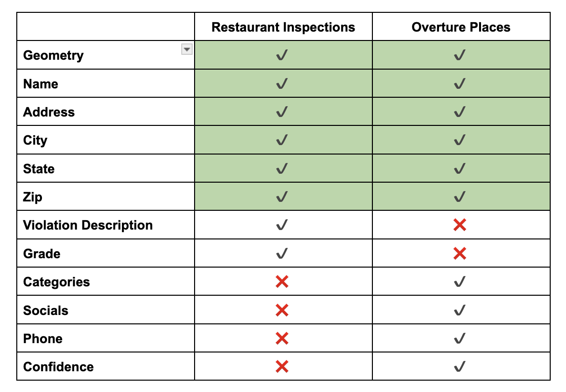
Using these common attributes, and a bit of SQL, we can quickly spin up a quick matcher using DuckDB.

Staging our datasets

With our inspection data saved as inspection_records.geojson, let’s boot up DuckDB, specifying a local database as a cache.

$ duckdb inspection_match.ddb

We’ll load the spatial and httpfs plug-ins, then load our inspections into a local table.

D install spatial;
D load spatial;
D install httpfs;
D load httpfs;
D CREATE TABLE IF NOT EXISTS inspections AS SELECT * FROM ST_Read('inspection_records.geojson');

Since there are multiple inspections for each venue, and we want to match each venue to an Overture Place, we’re going to create a separate table just for the facilities.

D CREATE TABLE IF NOT EXISTS facilities AS 
  SELECT Facility_ID, Facility_Name, Address, City, State, Zip, geom
  FROM inspections
  GROUP BY Facility_ID, Facility_Name, Address, City, State, Zip, geom;

note

We’re only pulling in each facility's ID and the columns which overlap with Overture’s Places.

Geospatial matching processes can get quite complex, so we’re going to load the Overture data we need in a local table before attempting any joins.

D CREATE TABLE IF NOT EXISTS places AS 
  WITH bounding_box AS (
    SELECT max(ST_Y(geom)) as max_lat, 
           min(ST_Y(geom)) as min_lat, 
           max(ST_X(geom)) as max_lon, 
           min(ST_X(geom)) as min_lon
    FROM facilities
  )
  SELECT 
    id, 
    upper(names['primary']) as Facility_Name, 
    upper(addresses[1]['freeform']) as Address, 
    upper(addresses[1]['locality']) as City, 
    upper(addresses[1]['region']) as State, 
    left(addresses[1]['postcode'], 5) as Zip, 
    geometry as geom, 
    categories,
    confidence 
  FROM (
    SELECT * 
    FROM read_parquet('s3://overturemaps-us-west-2/release/2025-03-19.1/theme=places/type=place/*', filename=true, hive_partitioning=1),
      bounding_box
    WHERE addresses[1] IS NOT NULL 
      AND bbox.xmin BETWEEN (bounding_box.min_lon - 0.01) AND (bounding_box.max_lon + 0.01)
      AND bbox.ymin BETWEEN (bounding_box.min_lat - 0.01) AND (bounding_box.max_lat + 0.01)
  );

We’re doing several things here that are worth breaking down:

1. We create a bounding box by computing the maximum and minimum latitude and longitude values of our inspections. This ensures we’re only pulling Overture Places relevant to our input dataset.
2. Our following SELECT statement prepares the Places data to more closely align with the conventions of our inspections data: the addresses column is broken down into component columns and we use only the primary name from the names column and label it to match Facility_Name.
3. Finally, we obtain the data from the Overture S3 bucket by remotely reading the parquet. A WHERE statement limits our request to a slightly buffered bounding box (buffered to ensure we’re capturing places near those facilities on the edges of our dataset).

We now have three tables: inspections with 27,515 records, facilities with 4,340 records, and places with 73,985 records.

Before we work on connecting them, we’ll add some spatial indexes to each table, making our lookups much faster:

D CREATE INDEX IF NOT EXISTS idx_places_geometry ON places USING RTREE (geom);
D CREATE INDEX IF NOT EXISTS idx_facilities_geometry ON facilities USING RTREE (geom);

Matching our data

Geospatial matching can be a simple or very complicated process. A simple join might just be a couple WHERE statements, while a complicated process might employ a compound pipeline with Bayesian comparisons, vector search, LLMs, and/or human reviewers. It all depends on your use case.

Geospatial matching can also be greedy or cautious. A greedy matching routine will have less stringent standards and err towards making mismatches, whereas a cautious match will apply strict standards and err towards missing a correct match.

What type of match you employ — simple or complicated, greedy or cautious — requires you to understand how your data is being used, the cost of a false positive, and more. This is to say: it’s a decision beyond the scope of this tutorial.

For our example, we will be constructing a simple cautious matcher. We’ve chosen to build a cautious matcher because our data describes inspection scores and violations; the cost of a false match is high. It is safer for us to show no health score than show a failing one for a restaurant that did not fail.

But to get started, we will write a join using three conditions with very loose thresholds. We’ll break down each condition below.

D SELECT 
    f.Facility_ID as input_id, 
    f.Facility_Name as input_name, 
    f.Address as input_address, 
    p.id as match_id, 
    p.Facility_Name as match_name, 
    p.Address as match_address,
    p.confidence as overture_confidence,
    ST_Distance_Sphere(f.geom, p.geom) as distance, 
    jaro_winkler_similarity(f.Facility_Name, p.Facility_Name) as name_similarity, 
    jaro_winkler_similarity(f.Address, p.Address) as address_similarity
  FROM facilities f
  JOIN places p
    ON ST_DWithin(f.geom, p.geom, 0.001)
    AND jaro_winkler_similarity(f.Facility_Name, p.Facility_Name) > 0.7
    AND jaro_winkler_similarity(f.Address, p.Address) > 0.8
  ORDER BY f.Facility_ID, distance;

Scanning down to the JOIN statement, we are using three comparisons to associate our records:

1. Is it close by? ST_DWithin(f.geom, p.geom, 0.005): This matches records if they’re within ~100 meters from each other (this is what 0.001 roughly equates to in our SRID)

2. Do the names match? jaro_winkler_similarity(f.Facility_Name, p.Facility_Name) > 0.7: This is a string comparison function that generates a score from 0.0 to 1.0, with 1.0 being an exact match. Here we’re comparing the listed name for each record. We’ve chosen the Jaro-Winkler metric because it weights the beginning of strings higher than the end of strings, which tends to work well here.

3. Do the addresses match? jaro_winker_similarity(f.Address, p.Address) > 0.8: We’re using the same function as the previous comparison, just with a slightly higher threshold, to compare our addresses.

With just this query, we can get pretty far. There are three levers — the values specified for each of the three statements above — that we can tweak until we’re close to good.

At this point, it’s helpful to look at the data yourself. I usually use DuckDB’s CSV export function and scan the results, looking for patterns to inform tweaking our parameters.

For example, here are 3 candidate Overture Places which match with “Thornhill Coffee Shop”, located at 5772 Thornhill Drive.

Name	Address	Distance	Name Similarity	Address Similarity
THORNHILL COFFEE HOUSE	5772 THORNHILL DR	35.52	0.96	1.00
THORNHILL SALON	5736 THORNHILL DR	41.46	0.85	0.93
THORNHILL PET HOSPITAL	5745 THORNHILL DR	70.93	0.87	0.93

Here, everything is functioning as it should be. Even though our matcher is looser (it’s letting in the two wrong candidates), the distance, name similarity, and address similarity metrics allow us to easily order our results and allow the correct record to bubble up.

But elsewhere, this is not the case. Consider this example for matches with “West Oakland Senior Center”, 1724 Adeline Street:

Name	Address	Distance	Name Similarity	Address Similarity
WEST OAKLAND BRANCH	1801 ADELINE ST	55.85	0.87	0.88
WEST OAKLAND JOB RESOURCE CENTER	1801 ADELINE ST	56.17	0.90	0.88
WEST OAKLAND SENIOR CENTER	1724 ADELINE ST	64.24	1.0	1.0

In this example, ranking in descending order of distance puts the correct match at the bottom. This cluster of match candidates suggests a perfect match for name and address should overrule slight distance differences.

Reviewing these cluster candidates is essential work when building a matcher. As you plot and peruse them, patterns will emerge, enabling you to better tune your parameters.

For larger matches — beyond the scale of ~4,000 restaurants in a single county — we recommend building evaluation test sets: human-verified correct and incorrect match pairs for a sample of your data. With an evaluation test set, one can more systematically tweak their matcher and quantitatively measure their performance.

But for our restaurant app scenario, we’re fine with a quick match to populate our listings. After reviewing the data and running a few adjusted queries, we landed on an effective simple conservative matcher query:

WITH ranked_matches AS (
SELECT 
    f.Facility_ID as input_id, 
    f.Facility_Name as input_name, 
    f.Address as input_address, 
    p.id as match_id, 
    p.Facility_Name as match_name, 
    p.Address as match_address,
    p.confidence as overture_confidence,
    ST_Distance_Sphere(f.geom, p.geom) as distance, 
    jaro_winkler_similarity(f.Facility_Name, p.Facility_Name) as name_similarity, 
    jaro_winkler_similarity(f.Address, p.Address) as address_similarity,
    ROW_NUMBER() OVER (
      PARTITION BY f.Facility_ID
      ORDER BY jaro_winkler_similarity(f.Facility_Name, p.Facility_Name) DESC
    ) as rank
  FROM facilities f
  JOIN places p
    ON ST_DWithin(f.geom, p.geom, 0.001)
    AND jaro_winkler_similarity(f.Facility_Name, p.Facility_Name) > 0.89
    AND jaro_winkler_similarity(f.Address, p.Address) > 0.75
)
SELECT * FROM ranked_matches WHERE rank = 1

This query yields 2,358 correct matches and no false positives, for a match rate of 55%. By adding more conditionals and stages, we could get much higher results (if you’d like the details about that, check out a longer exploration here), but for our restaurant listing app, this suits our needs.

Enriching data with GERS IDs & producing a bridge file

Enriching our table

With our matcher written and tuned, let’s add a column to our facilities table named gers_id and populate it with our join query above:

ALTER TABLE inspections ADD COLUMN geometry VARCHAR;
ALTER TABLE inspections ADD COLUMN gers_id VARCHAR;
WITH ranked_matches AS (
    SELECT 
        f.Facility_ID as input_id, 
        f.Facility_Name as input_name, 
        f.Address as input_address, 
        p.id as match_id, 
        p.Facility_Name as match_name, 
        p.Address as match_address,
        p.confidence as overture_confidence,
        ST_Distance_Sphere(f.geom, p.geom) as distance, 
        jaro_winkler_similarity(f.Facility_Name, p.Facility_Name) as name_similarity, 
        jaro_winkler_similarity(f.Address, p.Address) as address_similarity,
        ROW_NUMBER() OVER (
            PARTITION BY f.Facility_ID
            ORDER BY jaro_winkler_similarity(f.Facility_Name, p.Facility_Name) DESC
        ) as rank
    FROM facilities f
    JOIN places p
        ON ST_DWithin(f.geom, p.geom, 0.001)
        AND jaro_winkler_similarity(f.Facility_Name, p.Facility_Name) > 0.89
        AND jaro_winkler_similarity(f.Address, p.Address) > 0.75
),
selected_matches AS (
    SELECT input_id, match_id FROM ranked_matches WHERE rank = 1
)
UPDATE inspections i SET gers_id = sm.match_id FROM selected_matches sm WHERE i.Facility_ID = sm.input_id;

Our facilities table is now enriched with GERS identifiers.

We can use this association to connect county health scores with our Overture Places basemap, then display them to our app users.

Further, if we can share our association with others, allowing them to benefit from the hard work we’ve done matching this data and easily connect it to their GERS-associated datasets using only a column join. One way to facilitate this is a bridge file.

Producing a bridge file

A bridge file is a join table, connecting GERS identifiers with another set of identifiers. Overture produces bridge files for the data sources we use to produce our datasets, allowing others to understand the provenance of our data and to quickly enrich their own data with Overture datasets, if they’re currently using one of our input data sources.

Once you’ve enriched your dataset with GERS identifiers, you can produce a bridge file like this:

SELECT Facility_ID, gers_id FROM inspections WHERE gers_id IS NOT NULL GROUP BY Facility_ID, gers_id;

Output this query as a CSV or parquet file and you’re done. It looks like this:

Facility_ID,gers_id
FA0319719,08f28346e8ca018503160340e65ac7b6
FA0319719,08f28346e8ca018503160340e65ac7b6
FA0319719,08f28346e8ca018503160340e65ac7b6
FA0002404,08f283098d6527200394e5ac0b19dbf5
FA0002404,08f283098d6527200394e5ac0b19dbf5

Performing a maintenance match

Associating with every monthly release

Overture currently releases a new version of its data every month. Our releases page specifies its location and provides release notes.

Geospatial data never sleeps. The real world is constantly changing, and in our case, restaurants are continually being opened and closed. Further, as Overture onboards new sources of data, the quality and coverage of our releases improves.

tip

Regularly associating your data with Overture’s is considered best practice.

While rerunning a match for our ~4,000 restaurants is relatively quick, larger dataset associations can be quite costly. Thankfully, there are a few things we can take advantage of to make this process easier.

Overture data changelog

With each data release, Overture generates a data changelog to capture changes in the data tied to the GERS ID for each feature. This information can be used to help reduce the scope of our maintenance match by identifying associated GERS IDs which have changed.

Using our same DuckDB database, we can remotely query the current changelog using a bounding box defined by our inspections dataset.

But wait — using the current March changelog won’t yield very interesting results, since we’ve already matched against the March data. For this exercise we’ll redo our work above, this time referencing the previous, February, Overture release.

Finding a Subset of Records That Need Matching

Matching against the February data, we connect 2,366 of our facility IDs to GERS IDs. Let’s see how the March changelog can help during our maintenance match.

First, we’ll cache the changelog in a table, filtered again by a bounding box:

CREATE TABLE IF NOT EXISTS changes AS
WITH bounding_box AS (
    SELECT max(ST_Y(geom)) as max_lat, min(ST_Y(geom)) as min_lat, max(ST_X(geom)) as max_lon, min(ST_X(geom)) as min_lon
    FROM facilities
)
SELECT 
    * 
FROM (
    SELECT id, bbox, filename, change_type, theme 
    FROM read_parquet('s3://overturemaps-us-west-2/changelog/2025-03-19.1/theme=places/type=place/change_type=*/*', filename=true, hive_partitioning=1),
            bounding_box
    WHERE 
        bbox.xmin BETWEEN (bounding_box.min_lon - 0.01) AND (bounding_box.max_lon + 0.01) AND
        bbox.ymin BETWEEN (bounding_box.min_lat - 0.01) AND (bounding_box.max_lat + 0.01)
);

This loads 87,229 records, which we’ll now intersect with our existing, associated GERS IDs:

SELECT Facility_ID, gers_id, change_type FROM inspections i 
JOIN changes c
ON i.gers_id = c.id
GROUP BY Facility_ID, gers_id, change_type;

Of our 2,366 associated GERS, 61% are unchanged. 37% have had data_changed, in some form or another, but Overture’s matchers have determined their GERS ID should persist – indicating that the record refers to the same entity.

But ~1.5% of our matched GERS IDs – or 37 records – have been removed. This could indicate a business has closed or a data record was identified as incorrect. Either way, this is a very small subset of records that we should rematch.

Given our use case and our desire to produce a cautious match, we will also be rematching against the data_changed records. There are many cases where a data update could correct an over-eager match based on incorrect input data.

For our county restaurant inspection use case, our data volumes aren’t of a sufficient size to really bother with this nuance (it’s easier to just rematch against the new release and quickly compare the output to make sure nothing is breaking). But for much larger datasets, where matching routines might take hours, this list of removed and data_changed records is valuable.

Let’s build a new query which finds the subset of the Facility_ID we should rematch. It’s similar to our last one:

SELECT Facility_ID, gers_id, change_type FROM inspections i 
LEFT JOIN changes c
ON i.gers_id = c.id
WHERE change_type IS NULL OR change_type IN ['removed', 'data_changed']
GROUP BY Facility_ID, gers_id, change_type;

We’re using a LEFT JOIN in this query to find the Facility_IDs which don’t have associated GERS IDS (hence, they might match with a new Overture release) and only selecting those matched records where the associated GERS ID has been removed.

This gives us 2,804 facilities we need to match.

To simplify our SQL, we’ll save the results from the above query as facilities_to_match.

Matching Unmatched records to the latest release

Armed with a shopping list of unmatched facilities, we can now drop our places table and refresh it with the March Overture data, then create our spatial index.

D DROP TABLE places;
D CREATE TABLE places AS 
  WITH bounding_box AS (
    SELECT max(ST_Y(geom)) as max_lat, min(ST_Y(geom)) as min_lat, max(ST_X(geom)) as max_lon, min(ST_X(geom)) as min_lon
    FROM facilities
  )
  SELECT 
    id, 
    upper(names['primary']) as Facility_Name, 
    upper(addresses[1]['freeform']) as Address, 
    upper(addresses[1]['locality']) as City, 
    upper(addresses[1]['region']) as State, 
    left(addresses[1]['postcode'], 5) as Zip, 
    geometry as geom, 
    confidence,
    categories 
  FROM (
    SELECT * 
    FROM read_parquet('s3://overturemaps-us-west-2/release/2025-03-19.1/theme=places/type=place/*', filename=true, hive_partitioning=1),
            bounding_box
    WHERE addresses[1] IS NOT NULL AND
        bbox.xmin BETWEEN (bounding_box.min_lon - 0.01) AND (bounding_box.max_lon + 0.01) AND
        bbox.ymin BETWEEN (bounding_box.min_lat - 0.01) AND (bounding_box.max_lat + 0.01) AND
        confidence > 0.3
);
D CREATE INDEX IF NOT EXISTS idx_places_geometry ON places USING RTREE (geom);

Finally, we run our match query again, limiting it to only those facilities in facilities_to_match.

WITH ranked_matches AS (
    SELECT 
        f.Facility_ID as input_id, 
        f.Facility_Name as input_name, 
        f.Address as input_address, 
        p.id as match_id, 
        p.Facility_Name as match_name, 
        p.Address as match_address,
        p.confidence as overture_confidence,
        ST_Distance_Sphere(f.geom, p.geom) as distance, 
        jaro_winkler_similarity(f.Facility_Name, p.Facility_Name) as name_similarity, 
        jaro_winkler_similarity(f.Address, p.Address) as address_similarity,
        ROW_NUMBER() OVER (
            PARTITION BY f.Facility_ID
            ORDER BY jaro_winkler_similarity(f.Facility_Name, p.Facility_Name) DESC
        ) as rank
    FROM facilities f
    JOIN places p
        ON ST_DWithin(f.geom, p.geom, 0.001)
        AND jaro_winkler_similarity(f.Facility_Name, p.Facility_Name) > 0.89
        AND jaro_winkler_similarity(f.Address, p.Address) > 0.75
    WHERE f.Facility_ID IN (SELECT Facility_ID FROM facilities_to_match)
),
selected_matches AS (
    SELECT input_id, match_id FROM ranked_matches WHERE rank = 1
)
UPDATE inspections i SET gers_id = sm.match_id FROM selected_matches sm WHERE i.Facility_ID = sm.input_id;

907 records were matched with this query, resulting in 2,358 total GERS associations.

Summary

Geospatial matching is a pain. However, by matching against Overture data once through a polished script or pipeline, you can seamlessly join with any other Global Entity Reference System (GERS) associated datasets. This integration makes your data more accessible, accelerates onboarding processes, and expands usability across teams that have also matched against GERS.

By leveraging GERS associations, teams can share the results of complex matching efforts and significantly enhance data value through simplified connections to additional datasets.