Land cover is live
Mapmakers rejoice!
The May release of Overture Maps includes new high-resolution land cover data and new cartographic schema properties.
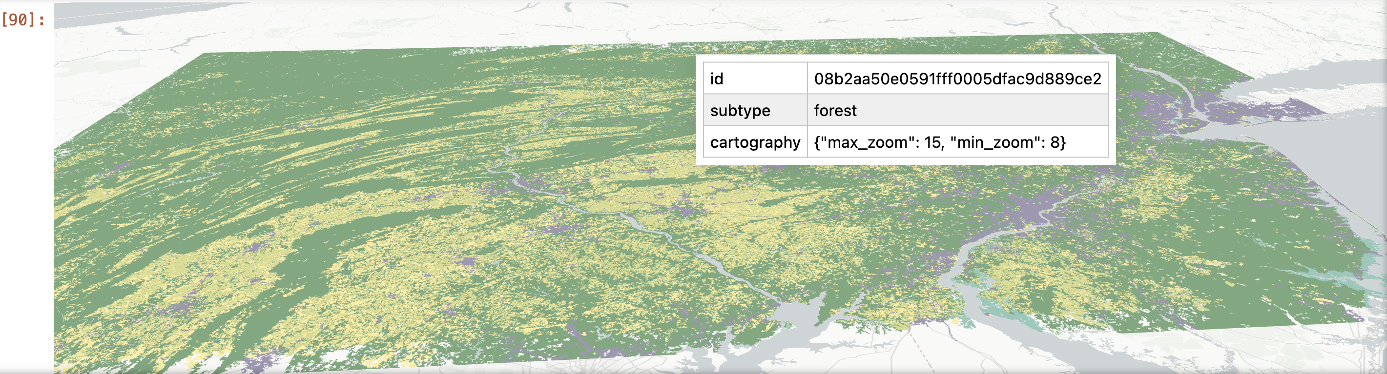
Our land_cover layer is vectorized data derived from the European Space Agency’s 2020 WorldCover (10m) rasters. It's similar to the land cover layer in the Daylight map distribution, but Overture Maps added higher-resolution data (zoom level 15) with more detail and land cover classes. You'll find 10 subtypes in the new data: snow, forest, urban, grass, crop, barren, wetland, moss, mangrove, and shrub.
Our May release also includes schema properties that offer cartographic "hints" for optimal use of Overture Maps data in mapmaking. We added min_zoom and max_zoom to define the recommended zooms for each resolution of land cover, using the common “slippy maps” zoom level specification. This is a first step toward improving the user experience for mapmakers. We plan to expand these properties in future releases of Overture Maps data.
Exploring land cover
In the notebook example below, we'll show you how to extract, process, and visualize land cover data for an area of interest using lonboard and the Overture Maps Python command-line tool. We recommend that you consult this example in the lonboard docs to better understand the methods used here. You can view and download the complete notebook on Notebook Sharing Space.
To follow along, you'll need to have JupyterLab or Jupyter Notebook running and the following dependencies installed:
import pandas as pd
import geopandas as gpd
import overturemaps
from shapely import wkb
from lonboard import Map, PolygonLayer
from lonboard.colormap import apply_categorical_cmap
# specify bounding box
bbox =  -78.6429, 39.463, -73.7806, 41.6242
# read in Overture Maps land_cover data type
table = overturemaps.record_batch_reader("land_cover", bbox).read_all()
table = table.combine_chunks()
# convert to dataframe
df = table.to_pandas()
# filter for higher resolution land_cover features
df_h = df[df.cartography.apply(lambda x: x['min_zoom'] == 8)]
# create color map for land_cover subtypes, loosely based on natural-color palette: https://www.shadedrelief.com/shelton/c.html
color_map = {
    "urban": [167, 162, 186],
    "forest": [134, 178, 137],
    "barren": [245, 237, 213],
    "shrub": [239, 218, 182],
    "grass": [254, 239, 173],
    "crop": [222, 223, 154],
    "wetland": [158, 207, 195],
    "mangrove": [83, 171, 128],
    "moss": [250, 230, 160],
    "snow": [255, 255, 255],
}
# apply color map to land_cover subtypes
colors = apply_categorical_cmap(df_h.subtype, color_map)
# dataframe to geodataframe, set crs
gdf = gpd.GeoDataFrame(
    df_h,
    geometry=df_h['geometry'].apply(wkb.loads),
    crs="EPSG:4326"
)
# create map layer
layer = PolygonLayer.from_geopandas(
    gdf= gdf[['id','subtype', 'cartography', 'geometry']].reset_index(drop=True),
    get_fill_color=colors,
    get_line_color=colors,
)
#render map
view_state = {
    "longitude": -76.2,
    "latitude": 39.6,
    "zoom": 8,
    "pitch": 65,
    "bearing": 5,
}
m = Map(layer, view_state=view_state)
m