Lonboard
In this example, we'll walk through three ways to fetch, process, and visualize Overture data in a Jupyter notebook using Lonboard and the overturemaps-py library. Lonboard is a Python library that makes visualizing large map datasets in Jupyter notebooks fast and efficient. It's built on GeoArrow and GeoParquet, which creates an opportunity for a fully binary workflow with Overture data.
Installation requirements
To follow along with these examples, you should have JupyterLab or Jupyter Notebook running and the following dependencies installed:
The examples below are available in the notebooks directory in our docs repository on GitHub.
Examples
Lonboard now has support for .from_duckdb() which allows us to interface directly with Overture data as Arrow tables and skip the steps with Shapely.
In the first and simplest example, we'll use the record_batch_reader method in the overturemaps-py library to load Overture GeoParquet data directly into a PyArrow table. Then we'll use lonboard's built-in visualization tools to create an interactive map.
GeoArrow
First, let's import our toolkit.
import overturemaps
from lonboard import Map, PathLayer
Next we'll get a bounding box for our area of interest.
# specify bounding box in Milan
bbox = 9.125034,45.433352,9.245223,45.507116
The record_batch_reader function accepts an Overture feature type and a bounding box as arguments. Note: .read_all() will load all of the requested bbox into memory, so it's wise to keep the bbox reasonably small.
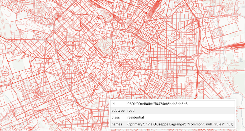
Let's grab some road data for Milan.
# need feature type and bounding box as arguments
table = overturemaps.record_batch_reader("segment", bbox).read_all()
We can inspect shape of the data.
table.shape
We can also dig into the complexity of the Overture transportation schema.
table.schema
Lonboard includes many built-in tools for visualizing map data. Here we're using PathLayer to render the segment features. Then we can set parameters for our interactive map display.
layer = PathLayer(
    table=table.select(["id", "geometry", "subtype", "class", "names"]),
    get_color=[200, 0, 200],
    width_min_pixels=0.4,
)

view_state = {
    "longitude": 9.18831,
    "latitude": 45.464336,
    "zoom": 12,
}
m = Map(layer, view_state=view_state)
m
GeoPandas
In the second example, we'll add a few steps in the notebook to convert the PyArrow table to a GeoPandas GeoDataFrame. Getting the data into a GeoDataFrame requires a few more tools, depending on which methods we use. Here's our expanded toolkit:
import overturemaps
import pandas
import geopandas as gpd
from shapely import wkb
from lonboard import Map, PolygonLayer
We'll use the same bounding box for Milan.
# specify bounding box
bbox = 9.125034,45.433352,9.245223,45.507116
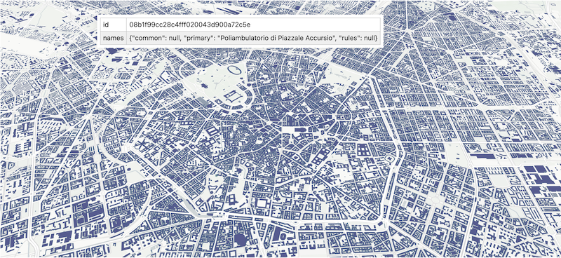
And we'll use the record_batch_reader method to pull the data into a PyArrow table. This time we'll grab buildings data.
# need feature type and bounding box as arguments
table = overturemaps.record_batch_reader("building", bbox).read_all()
table = table.combine_chunks()
Converting the table to a Pandas DataFrame is straightforward.
# convert to dataframe
df = table.to_pandas()
But we need an extra step to create the GeoDataFrame. Specifically we need to convert to the geometry to a Shapely geometry as we load into a GeoDataFrame.
# DataFrame to GeoDataFrame, set crs
gdf = gpd.GeoDataFrame(
    df,
    geometry=df['geometry'].apply(wkb.loads),
    crs="EPSG:4326"
)
We'll use Lonboard's PolygonLayer to render the buildings. The we'll set the parameters for our interactive map display.
layer = PolygonLayer.from_geopandas(
    gdf= gdf[['id', 'geometry', 'names']].reset_index(drop=True),
    get_fill_color=[93, 103, 157],
    get_line_color=[0, 128, 128],
)

view_state = {
    "longitude": 9.18831,
    "latitude": 45.464336,
    "zoom": 13,
    "pitch": 45,
}
m = Map(layer, view_state=view_state)
m
geodataframe method in overturemaps-py
In the last example, we'll use the geodataframe method in the overturemaps-py library to pull Overture data directly into a GeoDataFrame. This method handles all the conversions internally, making our lives easier and our notebooks cleaner.
Here's the toolkit:
import geopandas
from overturemaps import core
from lonboard import Map, ScatterplotLayer
Once again, we'll use the bounding box in Milan.
# specify bounding box
bbox = 9.125034,45.433352,9.245223,45.507116
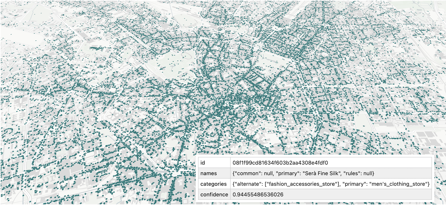
Direct to GeoDataFrame using the geodataframe method!
# read in Overture place feature type, direct to geodataframe
gdf = core.geodataframe("place", bbox=bbox)
Use ScatterplotLayer to render the point data and create an interactive map display in the notebook.
# create map layer
layer = ScatterplotLayer.from_geopandas(
    gdf,
    get_fill_color=[0, 128, 128],
    radius_min_pixels = 1.5,
)

view_state = {
    "longitude": 9.18831,
    "latitude": 45.464336,
    "zoom": 13,
    "pitch": 45,
}
m = Map(layer)
m
Next steps
- For a more complex example with Lonboard and Overture data, head over to the Lonboard docs.
- Check out the example with land cover data and Lonboard on our engineering blog.